Dynamic Pricing with RL: Balancing Margins & Profit

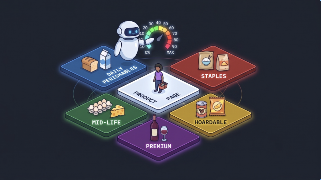
A from-scratch RL pricing engine, a simulated population of psychologically driven shoppers, and the training journey that eventually beat a hand-tuned heuristic engine.

Introduction

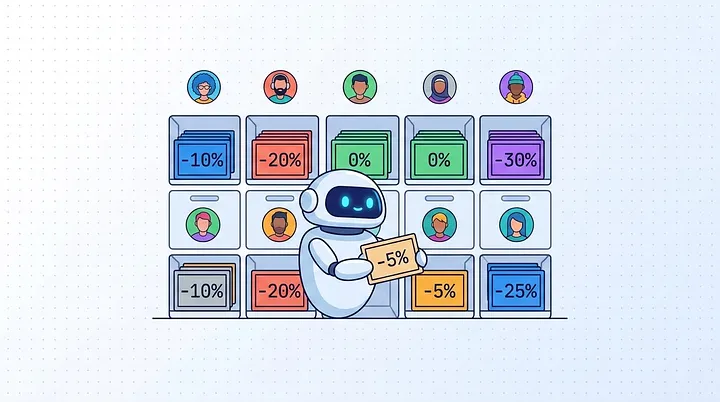
TL;DR — We trained a recurrent PPO agent to set grocery discounts in a simulated market of psychologically distinct shoppers. Rewarded on nothing but immediate margin, it learned to manage price anchors, retention, and spoilage well enough to beat a hand-engineered pricing heuristic by double digits — on products it had never seen. Here’s what worked, what broke, and the one architectural trick that mattered most.

Imagine a customer opens a product page for a carton of milk. You have one shot to decide what to charge them — not the shelf price everyone sees, but a discount tailored to this person, right now.

Offer too little discount, and a price-sensitive shopper shrugs and buys milk somewhere else. You keep your margin on a sale that never happened. Offer too big a discount, and you win the sale, but you’ve also taught this customer that milk “should” be cheaper than the original price. Next week, they’ll wait for the discount. The week after, they’ll expect a deeper one. You’ve quietly trained your own customer to erode your future margin.

That’s the trap at the center of personalized dynamic pricing. Every discount is three decisions at once:

• maximize conversion — get the sale today;
• protect margin — don’t give away more than you have to;
• don’t poison the future — keep the customer’s price expectations healthy.

The cruel part is that your feedback signal only tells you about today. You see the immediate sale and the immediate margin. The slow erosion of a customer’s price anchor, the customer who silently defects to a competitor, the perishable stock that spoils because you over-discounted and they over-bought — none of that shows up in the reward for this single transaction.

This is exactly the shape of a problem reinforcement learning is supposed to be good at: actions with delayed, tangled consequences. So we asked a concrete question:

Can an RL agent learn the hidden psychology of a shopper — price anchors, consumption rhythm, the fear of spoilage — from nothing but an immediate-margin reward, and beat a carefully hand-tuned pricing strategy?

To answer it, we built three things: a simulated marketplace, a population of fake-but-believable shoppers, and an RL agent that we trained, broke, and rebuilt a dozen times. This article is the story of that journey — including the parts that didn’t work, the one experiment we couldn’t afford to run, and the result that surprised us most.

Marketplace

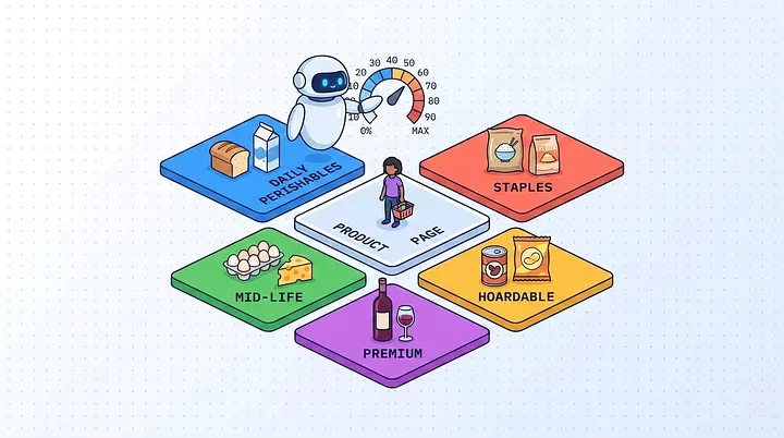
We modeled the environment as an online grocery store. The catalog is 25 products spread across five categories, deliberately chosen so that shelf life and margin pull in different directions:

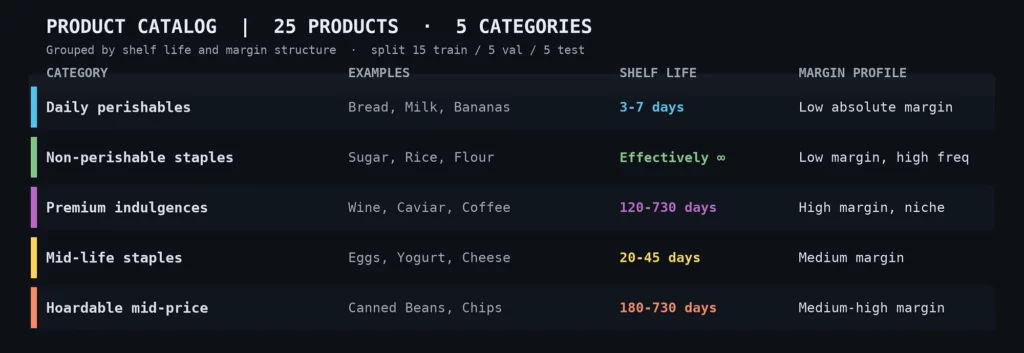
The products are split by hand across train / val / test sets, so each split contains all five categories. The agent is evaluated on products it has never seen during training.

Every time a user lands on a product page, the agent observes the situation and picks a discount. What does it see?

At a high level:

• user’s recent history (when they last visited, what discounts they took, how often they buy);
• product’s attributes (shelf life, maximum allowable discount).

There’s one deliberate twist in the observation design that becomes important later — the agent’s critic gets to see hidden information the actor never does. Hold that thought; it pays off in later sections (the full feature list is in Appendix A).

The action is a discount. Internally, the agent chooses from 11 discrete buckets—0%, 10%, 20%, up to 100% (by design, 100% represents the product’s maximum safe discount, which yields a $0 margin) — which are then applied as a continuous price. That “discrete vs continuous” choice sounds like a footnote. In reality, it turned out to be the single most important decision in the entire project.

Reward function

The reward is intentionally simple: the normalized margin on the transaction.

Dividing by retail price keeps the numbers comparable across wildly different products — a loaf of bread at $4 and a tin of caviar at $120 shouldn’t live on totally different reward scales (we will see later just how mandatory that normalization is).

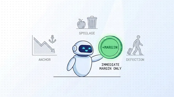
Important! The reward is purely immediate. There is no bonus for keeping a customer’s price anchor healthy. No penalty for causing spoilage. No term for retention or lifetime value. The agent is told only about the margin it earned on this transaction.

Everything that makes this problem hard — the anchor erosion, the defections, the spoilage — is absent from the reward. The bet we’re making is that a recurrent PPO agent, given enough history and the right architecture, will learn to manage those long-term trade-offs implicitly, simply because short-sighted greed gets punished a few steps down the line. The rest of this article is, in effect, the story of how that bet paid off.

Building humans: The LLM proxy

Before you can train a pricing agent, you need someone for it to sell to. We needed a population of shoppers who behave like people: who resent being overcharged, who stock up on a good deal, who let perishables spoil if they buy too much.

Our first instinct was the obvious modern one: use an LLM as a “human proxy”. It’s flexible, it’s zero-shot, and it lets you test behavioral hypotheses without writing a line of simulation logic.

So we tried the naive version first — a straight call. Pack the user’s situation into a single prompt (your inventory, the price, your budget personality) and ask: “How many units do you buy?”.

It failed consistently. The model would correctly notice the obstacles — “this price is high”, “this would exceed the shelf life” — and then talk itself into buying anyway. It hallucinated justifications for hoarding with remarkable creativity:

• using low inventory as an excuse to buy at any price;
• citing the need to maintain a “habit”;
• rationalizing a bad deal because it was “only a small amount” or a “cheap product anyway”.

Even though such behavior is native to some people, creating a pricing engine for this population would be too easy and wouldn’t add value to the community.

We could have mitigated this with few-shot examples or hard thresholds baked into the prompt — but that would just teach the model to copy our examples, and the organic, surprising behavior we wanted would collapse into overfitting.

The fix was to stop asking the model to make a decision in a single call. We split the decision into a push–pull chain:

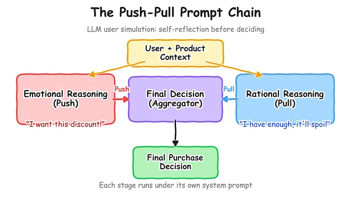
Forcing the model to articulate both sides before committing resolved the worst of the hallucinations. In addition, we added a couple of supporting tricks — for instance, hiding the exact inventory number when supply was only moderately low, so the model couldn’t lean on “I’m running out” as a lazy excuse.

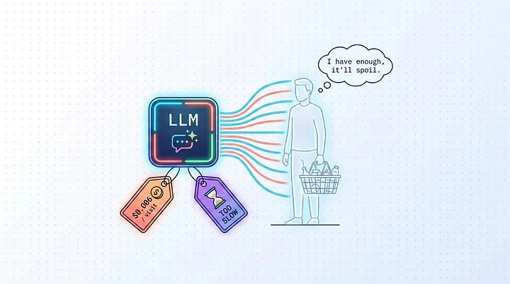
Eventually, it worked. We had believable shoppers. There was just one problem, and it was fatal for our actual goal: It was far too slow and too expensive.

A single user visit costs about $0.006, with gpt-5.4-nano in a low-reasoning setting. RL training needs millions of visits — at that rate, one million steps cost roughly $1,200 (using caching), and we need many millions. Local open-weight models dodge the dollar cost but are still orders of magnitude too slow to sit inside a training loop for the prototype.

The LLM gave us a believable model of shopper psychology. We just couldn’t afford to train against it. So we reverse-engineered it!

Building Humans: The Heuristic Twin

Introduction

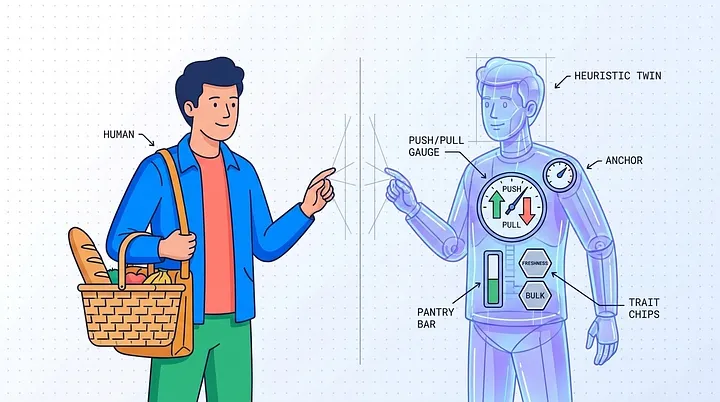
The idea: build a mathematical model that reproduces the LLM’s push–pull psychology, but runs thousands of times faster and costs nothing. Not a black box — a transparent system of competing forces that mirrors the tug-of-war inside a buyer’s head.

The grounding for who these shoppers are comes from a real source: NielsenIQ’s Global Consumer Outlook report. The behavioral traits and their prevalence are drawn from actual survey data — for example, the report finds that over half of consumers will pay more for fresh products, so half of our population carries a freshness-lover trait; roughly 30% stock up when there’s a promotion, so 30% are bulk-buyers, and so on across budget, planning, and inventory axes (of course, these are deliberate simplifications, not an academic population model — but they keep the simulation anchored to something real).

In our simulation, each shopper is assembled from seven behavioral traits — bargain-hunter, premium-seeker, price-careless, rational, impulsive, bulk-buyer, and freshness-lover — each switched on with a prevalence taken from the survey data. They fall along three axes: how a person reacts to price (a bargain-hunter chases every discount, a premium-seeker grows suspicious of one, a price-careless shopper barely looks), how they plan (rational vs impulsive), and how they stock up (bulk-buyer, freshness-lover). A user may have 0 or more traits.

Moreover, each simulated shopper is more than a bag of traits. On top of their personality, every user also carries:

• Loyalty score, drawn uniformly from [0.2, 1.0]. It does exactly one job: it sets how likely a price-insensitive shopper is to wander off to a competitor on any given visit.
• Personal visit rhythm. Not everyone shops on the same cadence, so each user gets their own visit window — its lower bound drawn from 2–14 days, its upper bound adding another 2–14 days of slack — and every visit is sampled fresh from that window. Across the whole population, visit gaps span 2 to 28 days.
• Per-product state — four randomized values for each product a user cares about: their interest-level (low / medium / high), how fast they consume it, how much they currently have in the pantry, and their starting price anchor. The same person can be a devoted milk-drinker with a stuffed fridge and a casual, anchor-less buyer of coffee.

This per-product/per-user state is what makes the population genuinely heterogeneous: two shoppers with identical personalities can still demand completely different pricing, simply because their pantries and consumption rates diverge.

Main logic

The purchase decision itself works on one item at a time. For each potential unit added to the cart, the model computes two opposing forces:

• Push = need + greed + convenience — the desire to buy;
• Pull = risk + resentment — the resistance to buying.

If push (plus a little noise) beats pull, the item goes in the cart, and we evaluate the next unit’s relevance. The moment the pull wins, the user stops. This naturally captures diminishing returns: the first carton of milk is easy to justify; the fifth one has to overcome much more accumulated resistance.

What’s inside those forces is where the psychology lives:

• Need grows as the user’s supply runs down toward their next expected visit;
• Greed is the thrill of a good deal relative to what they expect to pay, and different personalities respond differently. A bargain-hunter‘s joy grows explosively with discount depth; a premium-seeker actually gets suspicious of discounts that are too deep (“what’s wrong with it?”);
• Risk bundles the friction of spending money, the one-time hurdle of opening the wallet at all, and the very real fear of buying perishable food that will spoil before it’s eaten;
• Resentment is what you feel when the price is above your internal expectation. Users will tolerate being overpriced on vital, high-interest necessities (e.g., water, bread), but get easily offended and refuse to buy low-interest impulse items if the price is hiked.

Two pieces of this deserve to be highlighted because they’re the heart of the long-term game the RL agent has to learn.

The price anchor

Every user carries an internal sense of what a product should cost — their price anchor — and it drifts over time, just like human memory:

• Forgetting: between visits, the anchor decays back toward the normal retail price by about 1% per day. Don’t give a discount to a customer for a while, and their expectations will reset to normal.
• Learning: when they see a new price, the anchor moves toward it — quickly when the price is below their anchor (we love a bargain and adjust to it fast), and more stubbornly when it’s above (we resist price hikes). And it moves more if they actually bought than if they only looked.

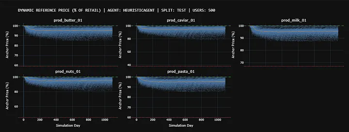
This single mechanic is why the problem is non-trivial. A deep discount today literally rewrites the customer’s expectations, lowering the margin you can earn tomorrow. An agent that optimizes only for today’s margin must discover this consequence through delayed feedback.

Spoilage

Between visits, the simulation ages each user’s inventory day by day: consumption is drawn down oldest-batch-first, shelf lives tick down, and anything that spoils or runs out is removed. Oversell a perishable, and the customer doesn’t thank you — they’re stuck with waste, and it suppresses their future buying.

Lost sales

There’s also an explicit lost-sale mechanism, which splits along personality lines. Price-insensitive shoppers (the price-careless and the premium-seekers) occasionally defect to a competitor purely at random, scaled by their loyalty — they needed the product, you didn’t capture it. Price-sensitive shoppers defect organically: their unmet daily consumption piles up as lost volume — a concrete count of exactly how much product they would have bought under reasonable pricing.

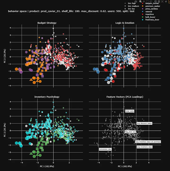
The payoff of building it this way is that, because every shopper is a different crossing of these traits and forces, the population doesn’t behave like one average blob. Distinct behavioral clusters emerge on their own.

Metrics & Evaluation

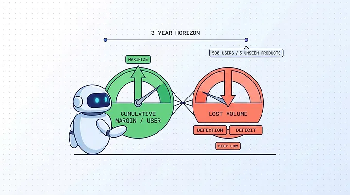
A single-step reward tells you almost nothing in a market like this — a deep discount can look great on this transaction and quietly wreck the next ten. So before comparing agents, we had to define two things: what we measure, and over how long.

Every agent is scored on a simulated 3-year horizon (1,095 days) over the held-out test split — 500 users and 5 products the agent never saw during training. Three years matter: it’s long enough for the slow dynamics — anchor erosion, spoilage, repeat-visit rhythms — to actually play out and separate a short-sighted policy from a patient one. A shorter run would flatter greedy agents that haven’t yet paid for the future damage they’re doing.

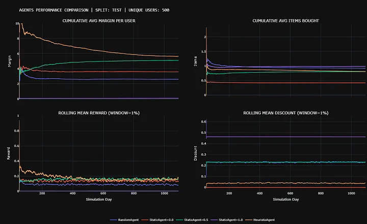
The metric that decides the leaderboard is Cumulative Mean Margin per User. This is the business bottom line, and it’s what every “+13%” in this article refers to: total margin earned, averaged across users and across time.

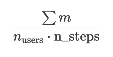
Where m is the margin per transaction:

In addition to the headline number, we track supporting telemetry to understand how an agent earns — or loses — its margin:

• Rolling Mean Reward per User — the raw RL step signal. Useful for watching training health, but far too myopic to rank strategies.
• Deal Count & Mean Deal Size — a behavioral fingerprint: does the agent nudge with frequent small discounts, or wait and trigger rare bulk buys?
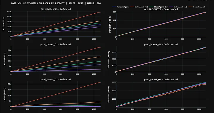
• Lost Volume — the metric that keeps greedy agents honest. It counts demand we failed to capture, in two flavors: defection volume (price-insensitive shoppers who wandered to a competitor) and deficit volume (price-sensitive shoppers whose pantry ran dry because our prices kept beating their expectations). This is the crucial counterweight to margin — a policy can post a healthy margin per sale and still be quietly bleeding volume.

The real objective lies in the trade-off between these two: maximizing cumulative margin while keeping lost volume low. Neither number alone tells you whether a pricing engine is any good.

Below are the metric samples for a set of our baselines (StaticAgent=X means that this agent always gives X*100% discount from the maximum safe one).

The Training Diary

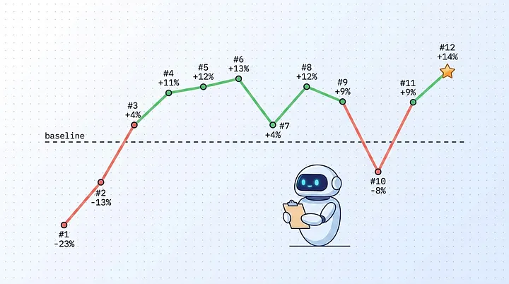
This is the part nobody usually shows you: not the polished final architecture, but the sequence of failures that led there. Each step below was a hypothesis, an implementation, and a result — and the failures taught us more than the wins.

The pre-recurrent failures #0. A standard continuous PPO agent, fed an averaged summary of the user’s last 50 steps through a linear network, fell apart — huge action variance and a critic that was effectively dead (EV ~0.08). The cause was structural, not a tuning issue: the environment stepped through different users on consecutive steps, so the agent saw its action on User A as causing User B’s next state — a broken MDP. Fixing the rollout buffer to process per-user trajectories revived the critic, but the linear network still couldn’t capture long-term history. That forced a structural rewrite.

Attempt #1 — Memory via Recurrent PPO. We migrated to an LSTM policy and rewrote the environment to simulate a single user-product pair in chronological order from start to finish. The critic stayed sharp (EV ~0.95) — but with a continuous action space, business performance was still poor (−23.37% compared to the HeuristicAgent baseline).

Attempt #2 — Asymmetric actor-critic. We let the critic see the 11 secret features while the actor stayed on the 5 public ones (the feature set grew in later attempts — Appendix A lists the final version). Still continuous, still below baseline (−12.89%) — but this is the seed of the payoff insight we return to later.

Attempt #3— The discrete breakthrough. Here was the core flaw of a continuous action space in this market: when the agent was torn between “0% to protect the anchor” and “50% to trigger a bulk buy”, it would output the average — a useless 25% that neither protected margin nor moved volume. The optimal actions were mutually exclusive extremes, and averaging them was the worst of both worlds. Switching to 11 discrete discount buckets forced the policy to commit to a categorical choice. This was the breakthrough: it was the first agent to beat the hand-tuned heuristic baseline on the test set at all (+4.20%).

Attempt #4— Statistical features + an honest distribution. Next, we fed the actor a few aggregated statistics about each user (their historical average discount, conversion patterns) so it didn’t have to reconstruct trends from raw history. At the same time, we switched to the realistic customer distribution (earlier, we’d quietly over-weighted bargain-hunters to persuade the agent into discounting — a hack we no longer needed). Combined, this lifted the agent to +11.08% over the heuristic.

Because both changes landed together, and they invalidated earlier checkpoints, we can’t fully separate how much credit goes to the features versus the distribution.

Attempt #5 — User repetition. We set user_repetitions=3, making the agent play against the same user several times in a row to strengthen its ability to exploit that profile’s long-term patterns. Marginal impact (+11.50% at 4M steps) — it became the asymmetric baseline for #7.

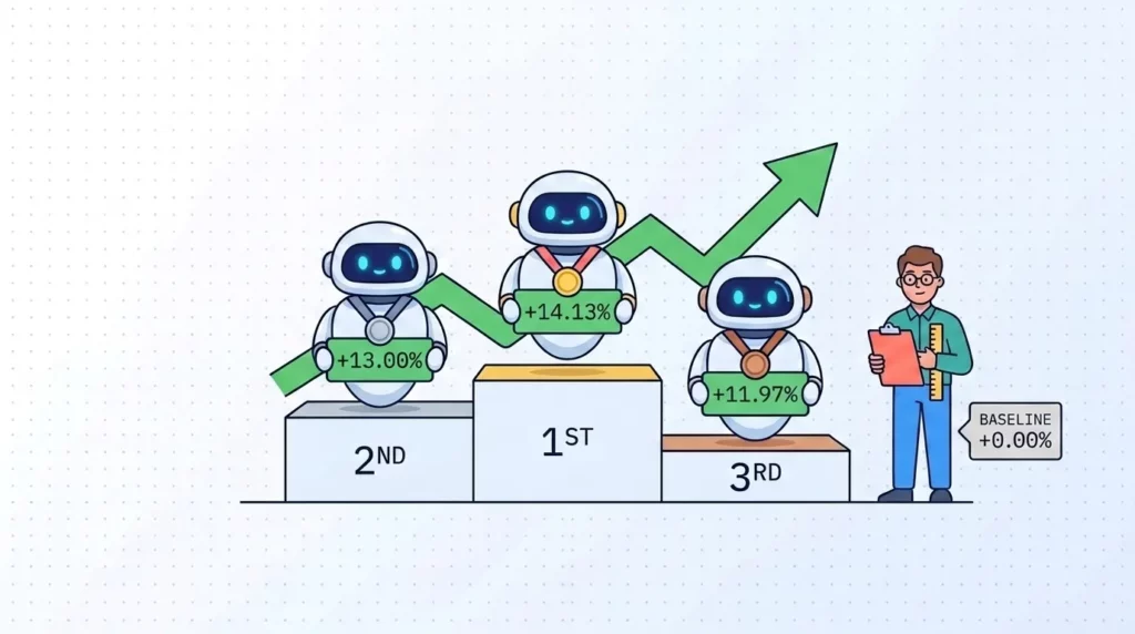
Attempt #6— Just train it longer. With the architecture finally sound, we suspected 4M steps were cutting the learning curve short. Doubling to 8M steps confirmed it: performance climbed to +13.00%.

With the architecture finally sound, the rest of the work was probing its boundaries — finding what helped, what didn’t, and what was load-bearing.

Attempt #7 — Fair critic. At this point, we experimented with how much value the asymmetric nature really gave to the agent. This experiment finished at +3.5% and is described in more detail in the next section.

Attempt #8 — A better-informed critic. Since the asymmetric critic was clearly carrying the team, we fed it even more: an explicit is_lost_sale flag in its secret observation, so it wouldn’t have to infer defections from inventory and price deltas. The result was underwhelming — +11.97%, no real lift over comparable models. The critic was apparently already deducing lost sales on its own. A small result, but a big hint for the next section.
Attempt #9 — More compute (20M steps). With 8M working so well, we pushed to 20M. It regressed to +9.02% — a clean case of policy overfitting to specific training trajectories. Past the sweet spot, more compute actively hurts (*of course, we could tweak the hyperparameters to make the agent more robust at longer training, but it wasn’t the end goal of our research).
Attempt #10 — Killing reward normalization. An ablation to see how load-bearing our per-product normalization really was: we removed the division by retail price and trusted the framework’s own running-variance scaling to cope. It collapsed to −7.88% — worse than the dumb static baselines. With prices from a few dollars to over a hundred, high-ticket items dominate the global variance; the advantage estimates for cheap high-volume products vanish, and the policy stops optimizing for the broader market. Static, domain-specific normalization is mandatory, not optional!
Attempts #11 → #12 — Product-category context. Finally, we gave the actor explicit context about what it was selling — a one-hot product category in the public observation. At 4M steps, it looked like a regression (+8.95%, #11): the richer input needed more time to converge. Running the same architecture for 8M steps (#12) confirmed it — and produced our global best, +14.13%. The same lesson as #6, sharpened: richer inputs only pay off if you pay for the training to utilize them.

Two of these attempts — the privileged-critic baseline (#5) and its blinded twin (#7) — deserve a closer look, because their gap is the most surprising result of the whole project. That’s the next section.

The Payoff Insight:

Secret Knowledge for the Critic

Remember the “twist” — that the critic sees information the actor doesn’t? This is where it earns its place, and it produced the most counterintuitive result of the project.

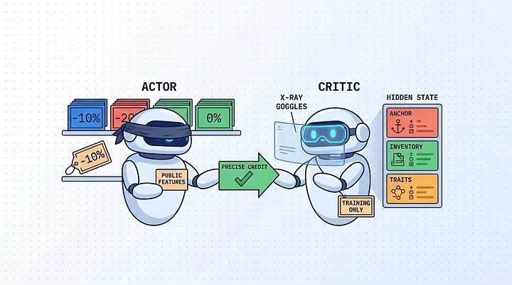
In an asymmetric actor-critic setup, the actor (which actually sets prices in production) sees only the public features — the stuff you’d realistically observe about a customer. But during training, the critic (which only estimates how good a state is, and is thrown away at deployment) is given the hidden truth: the customer’s real price anchor, their true inventory, their psychological traits. The actor still has to act blind; the critic just gets to grade it with full knowledge.

We ablated it: one model with the privileged critic (#5), one where the critic was blinded to the same public-only features as the actor (#7). The gap was large — roughly +11.5% versus +3.5%.

The counterintuitive part is why. You’d expect the blinded critic to be a much worse predictor… it wasn’t! Its explained variance was nearly identical to the privileged critic’s, both sitting in the 0.92–0.96 range. Both critics were excellent at predicting average returns.

The difference wasn’t prediction accuracy — it was gradient quality. The privileged critic, because it could see the hidden state, could assign credit precisely: it knew that offering a deep discount was brilliant specifically because this customer’s inventory had just hit zero, and forgettable otherwise. That precision produced sharper, more reliable learning signals, which in turn let the actor learn a genuinely targeted strategy — pinpoint discounts at the right moment — rather than retreating to a safe, averaged discount rate.

The lesson generalizes well beyond pricing: a critic that predicts averages well can still be a poor teacher. What you want from a critic isn’t just accuracy on the mean — it’s the ability to tell apart two superficially similar states that demand opposite actions. Privileged information during training buys you exactly that, even when it barely moves the accuracy number.

Benchmarks

Here’s the full leaderboard, every agent measured as relative margin against the hand-tuned heuristic (the 0% line).

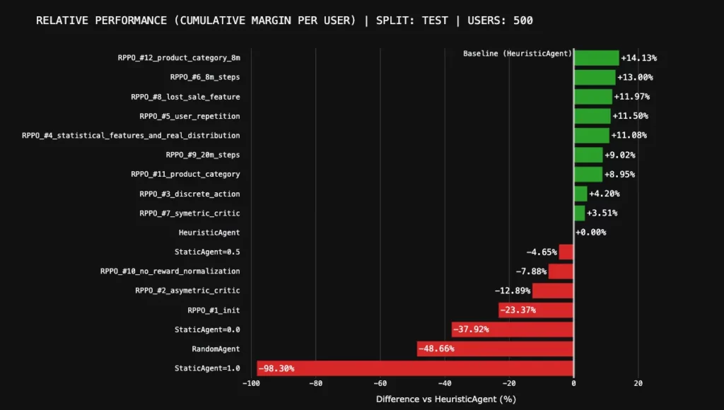
First, what the baselines tell us about the market itself:

• Never discounting is a disaster. StaticAgent=0.0 lands at −37.92%. Refuse to discount, and price-sensitive customers simply leak away to competitors. The market punishes pure greed.
• Randomly discounting is worse. RandomAgent at −48.66% confirms that throwing money around with no strategy shreds margin.
• But a dumb constant discount is shockingly good. StaticAgent=0.5 — a flat 50% off, forever, to everyone — sits at just −4.65%. That’s a humbling result: a strategy with zero intelligence captures enough volume to nearly match a sophisticated heuristic. It’s a strong local optimum, and it sets a reasonable baseline. The heuristic only beats it by carefully managing anchors and timing.
• And the bar itself isn’t naive. HeuristicAgent reconstructs each user’s hidden anchor, scales discounts to their consumption rhythm, and selects the depth using a robust UCB approach (Appendix B) — thereby defining the 0% reference line.

Second, let’s revisit our headline RL attempts:

• The early continuous agents (#1, #2) sit below even the dumb baseline, at −23.37% and −12.89% — the action-averaging penalty made concrete.
• The discrete breakthrough (#3) is the first to cross the line at +4.20%.
• Statistical features and the realistic distribution (#4) jump to +11.08%.
• More training time (#6) reaches +13.00%.
• And the global best — product-category context given enough training time (#12) — tops out at +14.13%.

Trained on nothing but immediate margin, the RL agent learned to manage anchor erosion and consumption timing well enough to beat a heavily engineered, domain-specific heuristic by double digits — on products it had never seen before.

But how well do we perform on the train / val sets?

Reassuringly well — the ranking we built over twelve attempts survives almost intact on unseen products: the strong agents stay in the double digits on both splits, the dead-ends stay underwater, and the baselines stay catastrophic. The order reshuffles slightly at the top, but that’s just noise from the small number of products per split, not a real regression. The gains generalize.

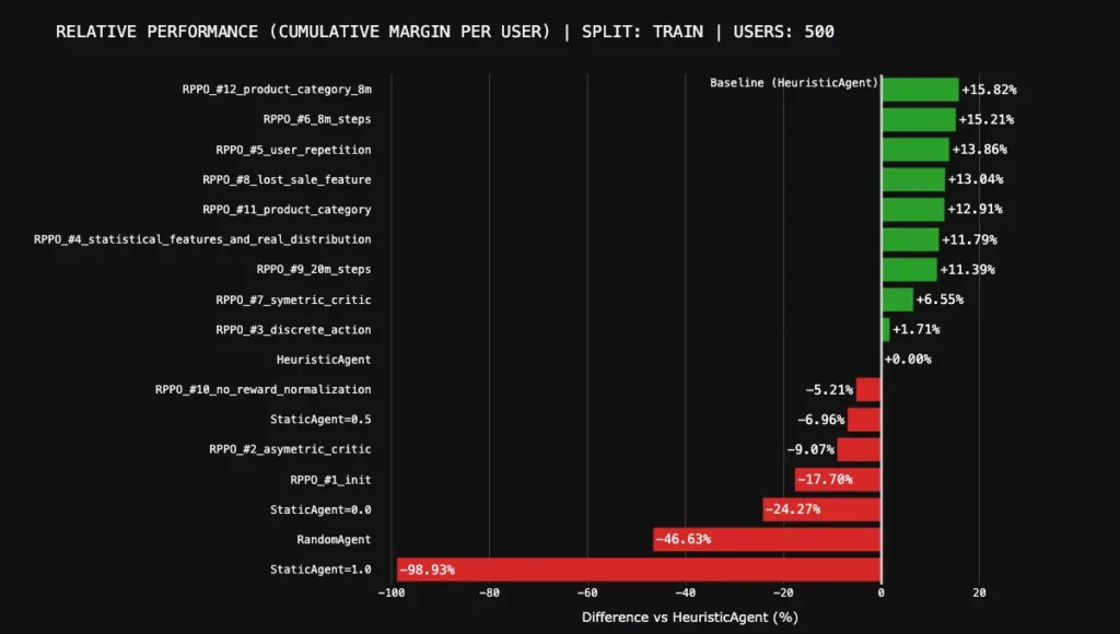
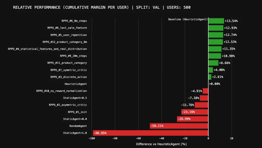
A note on statistical validity: across five evaluation runs, the heuristic’s cross-run variance was about 0.5%, so the environment itself is stable and these gaps are real market effects rather than evaluation noise.

Limitations and Next Steps

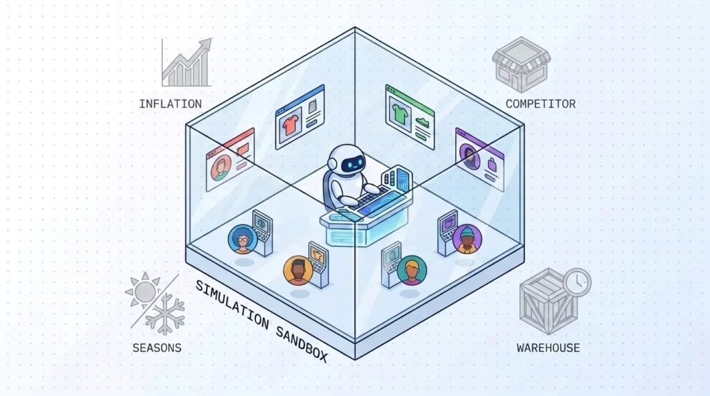
A few honest caveats, because a simulation is only as trustworthy as the assumptions you’re willing to name:

• Our shoppers are engineered, not fitted. The behavioral parameters are grounded in consumer-psychology survey data, but they were tuned by intuition, not fitted to a real retailer’s transaction logs. The goal was to prove RL can solve a complex delayed-reward pricing problem — not to build a digital twin of a specific grocery chain.
• We modeled the fairness question away. Hyper-personalized pricing carries real reputational risk. If a customer discovers they paid full price while a friend got 50% off the identical item, the strike can erase any margin you gained. Our agent optimizes in a social vacuum; a production system could not.
• Static macroeconomics. Retail and wholesale prices are fixed. We don’t model inflation, seasonal demand swings, or supply-chain shocks.
• Store-side inventory aging. In our world, a product’s shelf-life clock only starts after the customer buys it. We ignore warehouse-side batching — yet in real retail, the pressure to clear soon-to-expire stock on the shelf is one of the single biggest drivers of discounting strategy.
• Flat cost. We assume a flat per-item wholesale cost. Reality has economies of scale (higher volumes are cheaper per unit) and freshness (smaller, more frequent restocks keep shelves fresher and lift baseline conversion). Our flat-cost model abstracts all of that away.
• Defection is approximated, not emergent. Our “lost sale” mechanic uses tuned probabilities rather than a real competitor reacting to our prices.

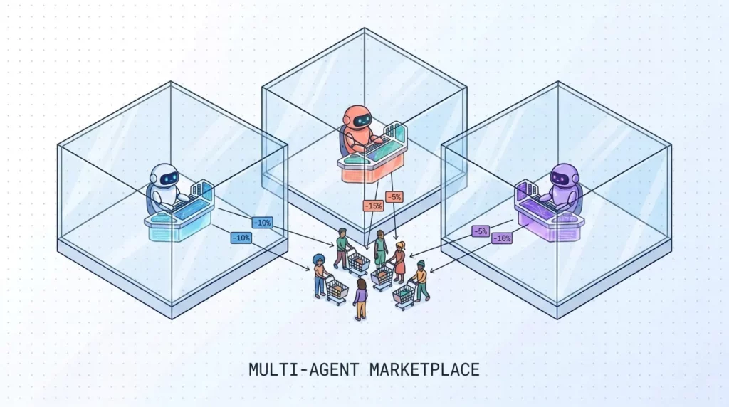
That last point is also the most exciting direction forward. The natural next step is a multi-agent marketplace: replace the scripted defection probability with actual rival pricing engines competing for the same customer’s limited wallet. Lost sales would then emerge organically from real competition rather than a preset number. Beyond that, we’d like to fit the shopper model to real transaction data instead of survey intuition, and upgrade the actor’s memory from an LSTM to a Transformer so it can infer hidden state — inventory, anchors — more sharply from raw history.

The bottom line

We set out to answer one question: can an RL agent learn the hidden psychology of a shopper — anchor memory, consumption rhythm, the fear of spoilage — from nothing but an immediate-margin reward and beat a hand-tuned expert?

Inside our simulation, the answer is yes. With no explicit reward shaping for anchors, retention, or spoilage, a recurrent PPO agent learned to manage all of them implicitly, beating a carefully engineered heuristic by double digits on products it had never seen before. Along the way, it taught us that the action space matters more than the algorithm, that reward normalization is load-bearing, that more compute can actively hurt without proper preparation, and — most surprisingly — that the most valuable thing you can give a critic isn’t accuracy, but privileged knowledge it can use to teach effectively.

While planning this article, we wanted to include the Heuristic vs LLM metrics on a dataset, but it turned out to cost more than we initially expected. That’s the next experiment, and we’ll report it straight when we run it. But the core bet — that reinforcement learning is flexible enough to absorb messy human pricing psychology on its own — held up.

Appendix A: Observation space

Public features [visible to both actor and critic]

• visit_gap_days / 365 — time between current and last visit, normalized;
• last_discount_offered / max_discount — discount offered, normalized;
• last_items_bought / max_items — purchase quantity, normalized;
• max_discount — product’s maximum allowed discount;
• shelf_life / 999 — product’s shelf life, normalized;
• days_since_last_purchase / 365 — recency of last purchase, not including last visit;
• purchase_frequency — purchases per observation window;
• mean_discount_taken — average discount at which purchases occurred per observation window;
• zero_discount_purchase_rate — fraction of full-price offers that converted per observation window;
• 5 product category flags: [perishable, staple, premium, mid-life, hoardable].

Secret features (visible only to critic — asymmetric information)

• inventory_days / shelf_life — how many days of supply the user has;
• reference_price / retail_price — the user’s internal price anchor;
• days_per_item / 30 — how many days one item lasts for this user;
• interest_level — encoded as 0.0/0.5/1.0 (low/medium/high);
• is_lost_sale — binary feature for price-insensitive customers;
• 7 binary character trait flags: [bargain-hunter, premium-seeker, price-careless, rational, impulsive, bulk-buyer, freshness-lover].

Appendix B: The Heuristic Agent

Because LLM evaluation is too slow for RL training, we needed a strong, hand-crafted mathematical baseline. The Heuristic Agent is not a simple rule-set; it is a sophisticated hybrid engine featuring continuous exploration and internal memory.

It consists of four distinct mechanisms:

1. Price Anchor Gatekeeper: The agent mathematically reconstructs the user’s internal price anchor based on past interactions (discount depth and whether a purchase occurred). If the user’s expected absolute discount exceeds a strict tolerance threshold (max_anchor_tolerance = 3% relative to the base retail price), the agent forces a 0% discount. This sacrifices immediate conversion to “heal” the anchor and restore long-term margin.
2. Heartbeat Detection (Natural Consumption Rhythm): The agent filters the user’s purchase history to find the 75th percentile of inter-purchase intervals, ignoring outliers. The mean of these clean gaps becomes the target_heartbeat — the estimated time it takes the user to consume their stash.
3. The Strike Zone & Early Probing: Discounts are only seriously considered when the user is within the “Strike Zone” (visits_since_last_buy >= heartbeat * 0.8). Outside this zone, the agent defaults to 0% but maintains a 5% exploration probability to update consumption rate estimates.
4. Continuous UCB Bandit: Within the strike zone, the agent evaluates 11 discrete discount buckets. For each bucket, it calculates the raw expected value:

Margin is strictly divided by the days until the next purchase, heavily penalizing deep discounts that remove the user from the market for months.

To account for future anchor damage, high discounts are explicitly penalized, and the final bucket is selected using the Upper Confidence Bound (UCB) formula:

Where:

• d is the discount bucket value;
• p is the discount_penalty_factor, representing future margin loss from price anchor degradation;
• c is the exploration constant ucb_exploration_c;
• N is the total number of evaluated historical strikes;
• n is the number of times this specific bucket was tried.

Finally, to transition from discrete buckets to our continuous environment, the agent injects Gaussian noise (std = 0.05) to the selected bucket.

___________________

You can find this article published on Medium. It was written by our Lead Data Scientist, Vlad Fliahin, in collaboration with our ML Engineer Maksym Arhunov.

you might also like…