Time Series Analysis and Sales Forecasting for Automotive

Introduction to Sales forecasting Engine

Time-series Sales forecasting is one of the most important topics in every business, helping to process data taken over a long period of time. Stock exchange, logistics, retail are classic industries where the ability to build predictive models becomes a crucial differentiator in a highly-competitive business environment. In our article we’ll try to explain how time series analysis and sales forecasting methods can be used for typical business tasks: finding hidden patterns, detecting trends in sales over the years, and predicting sales in the future.

Background Analysis

There are many time series forecasting models out there – from well-known and thoroughly studied, such as Naïve and Exponential Smoothing to the new and hot ones, like Facebook Prophet and LSTM models.

In the Naïve model, the forecasts for every horizon correspond to the last observed value and assume that the stochastic model generating the time series is a random walk. An extension of the Naïve model is called SNaïve (Seasonal Naïve), and this one assumes that the time series has a seasonal component.

Facebook Prophet is open-source software released by Facebook’s Core Data Science team. This model assumes that time series can be decomposed by the trend, seasonality, holiday, or error components.

LSTM stands for Long-Short Term Memories which come from the Neural Network domain. They are mostly used with unstructured data (e.g. audio, text, video), but may benefit from the transfer of learning techniques when applied to standard time series.

In this article, we would like to share with you our experience of using the SARIMA model. It works well for the car sales because of the sales seasonality and relative simplicity of this domain.

General Data Description 

The dataset contains the number of units and total sales of new motor vehicles, grouped by the vehicle type and the manufacturing location in Canada from 1946 to 2019, with data sampled on a monthly basis.

It is accessible here: Data Set

The initial data structure looks in the following way: 

There are 18 columns: 1 DateTime format, 5 numeric, 13 categorical.

After filtering the data by: Country, Vehicle type, Manufacturing Location, Seasonal Adjustment, and then dropping all columns, except for the two: REF_DATE and VALUE, we receive the final version of our dataset. It contains 888 rows, 1 numerical column and an index in the DateTime format:

Our time series is univariate, which means that:

• We are considering only the relationship between the y-axis value and the x-axis time points. 
• We don’t take into account any outside factors that may be affecting the time series.

Data Analysis

Time Domain Analysis

By means of a simple pandas command, we got the overall statistics for new cars sales in Canada between 1946 and 2019:

We quickly plot the data out with the matplotlib package, where y-axis stands for Sales, x-axis stands for years and then we’re able to make some conclusions:

• There is an upward trend over the years

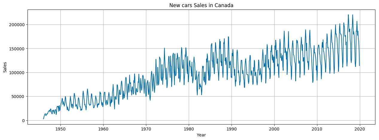
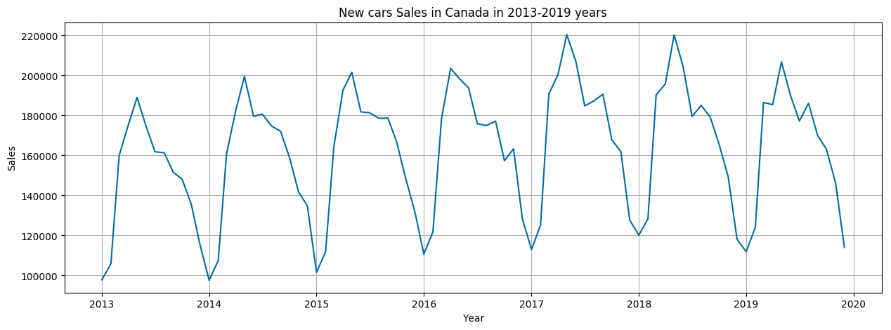
• Mostly, there is a slight upward trend within any single year.
• June and August show peaks in sales.
• November and December are the low seasons.

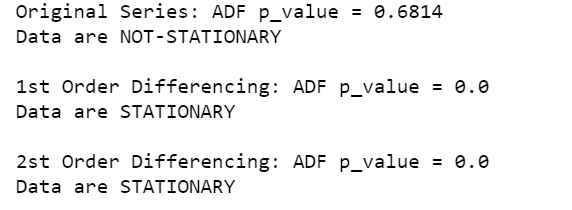
Stationarity Testing Using the Augmented Dickey-Fuller Unit Root Test

This is a statistical test that we run to determine if the time series is stationary or not.
The null hypothesis of the ADF test is that the time series is non-stationary. In other words, we have two options:

1. P-value is more than the significance level (0.05), which means that there is no sufficient statistical evidence to reject the null hypothesis.
2. here is sufficient statistical evidence to reject the null hypothesis, when p-value of the test is less than the significance level (0.05).

In our case, p-value = 0.6814 (which is more than 0.05), which means that we failed to reject the non-stationarity hypothesis.

Frequency (Seasonality) Analysis

We performed the seasonality analysis in order to find out the prominent frequencies (periodicity) in the frequency domain using the Fourier Transform for full-time series and the alternating component of the series. 

Here is the Energy Spectral Density (ESD) plot for new cars sales in Canada:

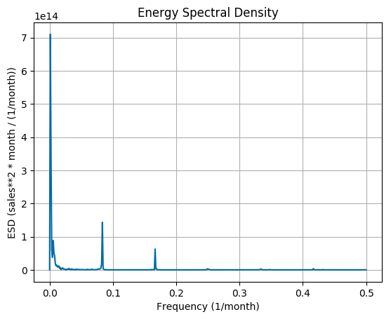
The maximum seasonality effects are at frequencies:
1, 2, 74 (1/month)

Periodicity:
96, 48, 1 (months)

Statistical Properties Analysis

Then, we conducted a statistical analysis to understand the probability distribution of data as well as to prove the normality of distributions. The histogram and the qq-plot of data examples are shown below.

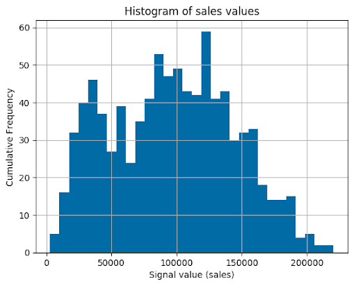
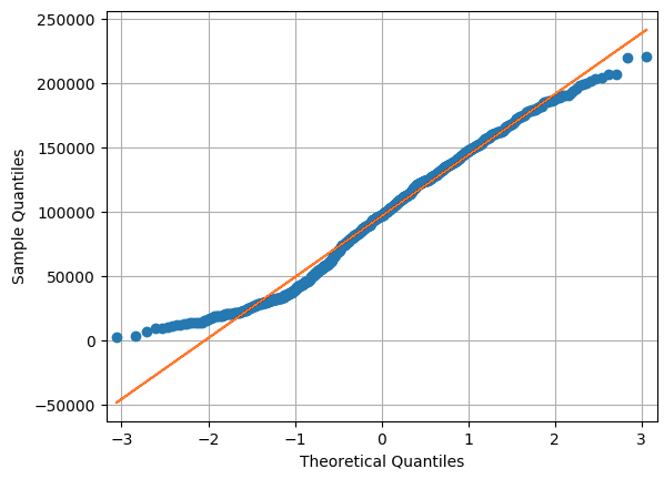
Normality Testing Using the D’Agostino and Pearson’s Test

This test helped us understand how far our data distribution is from the normal one by computing the p-value in hypothesis testing:

• null hypothesis – data are from the normal distribution
• alternative hypothesis – data are not from the normal distribution (p-value < 0.05)

Judging by the result of our p-value, we could draw the following conclusion – we have some strong enough evidence that the data distribution is not normal.

Method and Model Description

There is an upward trend, seasonality and some noise, so we can use the python package called  <statsmodels> to perform a decomposition of this time series. 

The decomposition of a time series is a statistical task that deconstructs the time series into several components, each representing one of the underlying pattern categories.

Our goal is to build a mathematical model to be able to forecast the future. 

Next, we decomposed the observed data (SEASONAL, TREND, and NOISE) with the following code:

As a result, we have  split the data into 4 components:

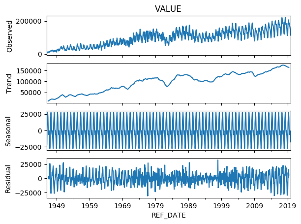
From the plot above two things come to light: 

• the seasonal component of the data 
• the obvious upward trend in the data

SARIMA is actually a bunch of simpler models combined into one complex model that can represent the time series by means of exhibiting its non-stationary properties and seasonality.

In theory, we have to find a set of coefficients p, d, q, P, D, and Q, which give us the lowest Akaike information criterion (AIC).

Moreover, for most years, the trend is rather linear while the seasonality and trend components are constant over time – so we choose an ADDITIVE model.

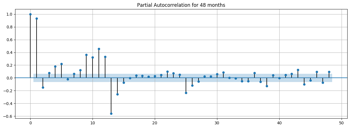
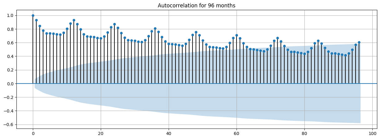
The first way of selecting this set of parameters is to take a look at the Autocorrelation, Partial Autocorrelation plots (ACF, PACF).

First, we have an autoregressive model AR(p). This is basically a regression of the time series onto itself. Here, we assume that the current value depends on its previous values with some lag. It takes a parameter p which represents the maximum lag. To find it, we look at the partial autocorrelation plot and identify the lag after which most lags are not significant.

In the example below, p would be 1.

After that, we add the order of integration I(d). The parameter d represents the number of differences required to make the series stationary. By means of differencing our time series up to the 2nd order, we see that the 1st order gave us stationary data:

Finally, we add the component: seasonality S(P, D, Q, s), where s is simply the length of a season. This component requires the parameters P and Q which are the same as p and q, but used for the seasonal component. Finally, D is the order of seasonal integration representing the number of differences required to remove seasonality from the series.

Combining these all, we get the SARIMA(p, d, q)(P, D, Q, s), model.

The main takeaway is: before modeling with SARIMA, we must apply transformations to our time series to remove seasonality and any non-stationary behaviors.

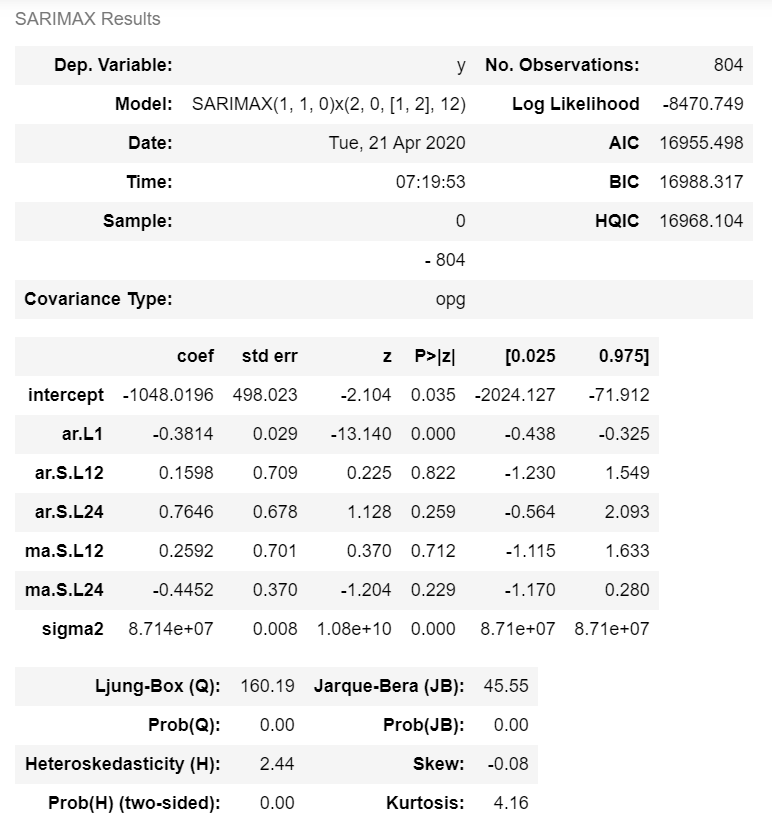
Another method (less time-consuming) is to perform a grid search over multiple values of p, d, q, P, D, and Q using some sort of performance criteria. By default, the AIC gives us a numerical value of the quality of each model, relative to each of the other ones. To be precise – the lower our AIC is, the better the model.

The pyramid-arima contains an auto_arima function that allows setting a range of p, d, q, P, D, and Q values and then fitting the models for all possible combinations. To get a summary of the best model we can use the following line of code:

Training 

The dataset was split into training and test sets, and then we trained the model by using the training data

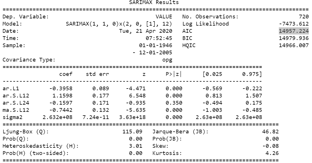
The best model parameters (SARIMAX(1, 1, 0)x(2, 0, 1, 12)) give us the lowest AIC:
AIC = 14957.224. 

Prediction and Evaluation

After our model has been fitted to the training data, we can try to forecast the future.

To get predictions about the future sales we can use the get_prediction() method of the model

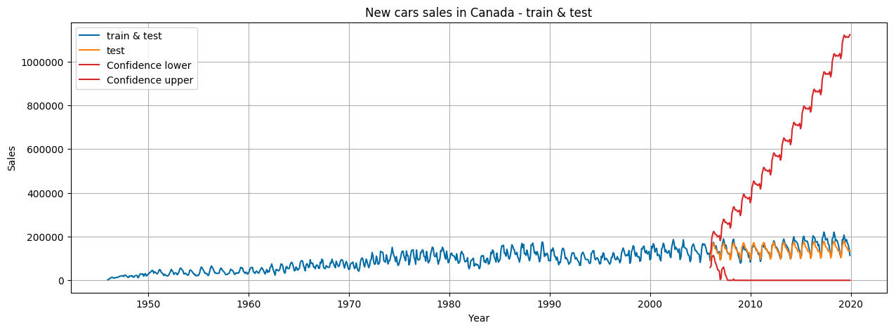
Here we plot our forecasted values to view how well our predictions match up with the test set with the real data:

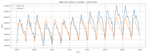
We can also just compare this to the entire data set to see the general context of our prediction

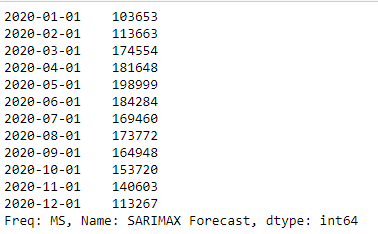
Let’s use the prediction to forecast the nearest 12 months (in our case – the whole year 2020):

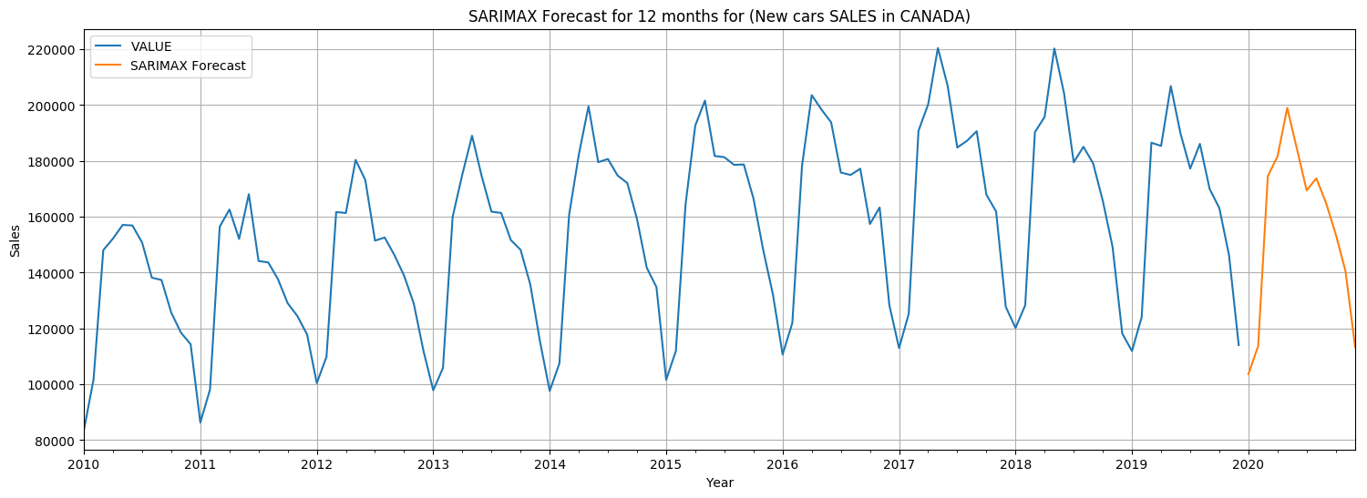
This is how the 12 months of 2020 are forecasted to look like:

In the forecasted data we see the same patterns as in the previous years:

• The worst months for sales are the first and the last months of the year, which totally makes sense in real life (Who thinks about buying cars before and after Christmas, right?)
• There is an upward trend with May being the first peak. Then, the trend goes down, with July being the bottom point.
• The second peak is in August, and the next downward trend culminates in December.

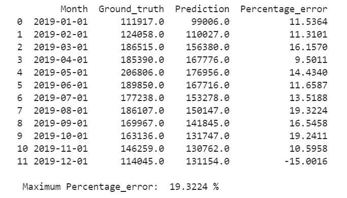
The last 20% of our data was used as a test set, on which we tested our model 

by standard metrics: MAE, MSE, RMSE, MPE.

Results

Discussion

The overall purpose of the study was to prove that it’s possible to efficiently forecast car sales using a simple statistical model. During our research we were able to prove that the SARIMA-based approach has acceptable outcomes. Such models can be easily implemented with various statistical software and their computational complexity is acceptable. Also, the approach has well-studied statistical properties. An important advantage of the described method is the ability to adapt to new conditions and time series properties by changing the coefficients. The Jupyter notebooks we used in our experiments are open-source and can be downloaded from the GitHub repository. [Sarima_new_cars_sales]

Limitations

Our only concern about the experiments is the well-known disadvantage of the SARIMA model. It can only extract linear relationships within the time series data. Predictions generated by the SARIMA model may not be suitable for complex nonlinear cases. It does not efficiently extract the full relationship hidden in the data. Another limitation is that the SARIMA model requires a large amount of data to generate accurate predictions.

Conclusions

The accuracy of the SARIMA predictive model in the form of MPE for car sales forecast has been obtained. It has been proved that the percentage error is not greater than 19.32 % for each of the 12 months ahead. Obviously, the accuracy of the model is high enough and the model can be used as a baseline for developing better models. The method is well suited for use in different business domains.

Acknowledgments

I want to thank my colleagues Andy Bosyi, Mykola Kozlenko, Alex Simkiv, Volodymyr Sendetskyi for their discussions and helpful tips as well as the entire Mindcraft.ai (MindCraft.ai: Data Science Development company | ML & AI Company) team for their constant support. Please share your own stories with Sales Forecasting tasks. 

References:

• SARIMA model
• Statsmodels package
• D’Agostino’s K-squared test – Wikipedia

you might also like…