Active Learning is a semi-supervised technique that allows labeling less data by selecting the most important samples from the learning process (loss) standpoint. It can have a huge impact on the project cost in the case when the amount of data is large and the labeling rate is high. For example, object detection and NLP-NER problems.
The article is based on the following code: Active Learning on MNIST

Data for the experiment

((4000, 28, 28), (4000,), (400, 28, 28), (400,))

<matplotlib.image.AxesImage at 0x7f59087e5978>

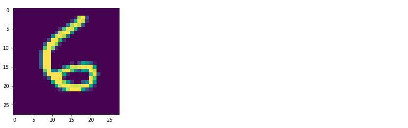
I will use a subset of MNIST dataset which is 60K pictures of digits with labels and 10K test samples. For the purposes of quicker training, 4000 samples (pictures) are needed for training and 400 for a test (neural network will never see it during the training). For normalization, I divide the grayscale image points by 255.

Model, training and labeling processes

As a framework, one can use the TensorFlow computation graph that will build ten neurons (for every digit). W and b are the weights for the neurons. A softmax output y_sm will help with the probabilities (confidence) of digits. The loss will be a typical “softmaxed” cross entropy between the predicted and labeled data. The choice for the optimizer is a popular Adam, the learning rate is almost default – 0.1. Accuracy over test dataset will serve as the main metric

Here I define these three procedures for more convenient coding.
reset() – empties the labeled dataset, puts all data in the unlabeled dataset and resets the session variables
fit() – runs a training attempting to reach the best accuracy. If it cannot improve during the first ten attempts, the training stops at the last best result. We cannot use just any big number of training epochs as the model tends to quickly overfit or needs an intensive L2 regularization.
label_manually() – this is an emulation of human data labeling. Actually, we take the labels from the MNIST dataset that has been labeled already.

Ground Truth

Labels:   4000              Accuracy:  0.9225

If we are so lucky as to have enough resources to label the whole dataset, we will receive the 92.25% of accuracy.

Clustering

<matplotlib.image.AxesImage at 0x7f58d033a860>

Here I try to use the k-means clustering to find a group of digits and use this information for automatic labeling. I run the Tensorflow clustering estimator and then visualize the resulting ten centroids. As you can see, the result is far from perfect – digit “9” appears three times, sometimes mixed with “8” and “3”.

Random Labeling

Labels:  400     Accuracy:  0.8375

Let’s try to label only 10% of data (400 samples) and we will receive 83.75% of accuracy that is pretty far from 92.25% of the ground truth.

Active Learning

Labels: 10          Accuracy:  0.38

[<matplotlib.lines.Line2D at 0x7f58d0192f28>]

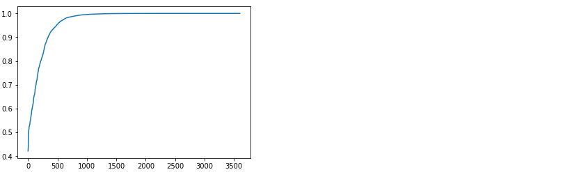
Now we will label the same 10% of data (400 samples) using active learning. To do that, we take one batch out of the 10 samples and train a very primitive model. Then, we pass the rest of the data (3990 samples) through this model and evaluate the maximum softmax output. This will show what is the probability that the selected class is the correct answer (in other words, the confidence of the neural network). After sorting, we can see on the plot that the distribution of confidence varies from 20% to 100%. The idea is to select the next batch for labeling exactly from the LESS CONFIDENT samples.

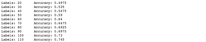
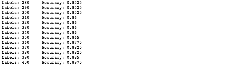
After running such a procedure for the 40 batches of 10 samples, we can see that the resulting accuracy is almost 90%. This is far more than the 83.75% achieved in the case with randomly labeled data.

What to do with the rest of unlabeled data

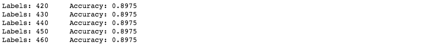
Labels:  4000    Accuracy: 0.8975

The classical way would be to run the rest of the dataset through the existing model and automatically label the data. Then, pushing it in the training process would maybe help to better tune the model. In our case though, it did not give us any better result.
My approach is to do the same but, as in the active learning, taking in consideration the confidence:

[<matplotlib.lines.Line2D at 0x7f58cf918fd0>]

Labels:   410        Accuracy:    0.8975

Here we run the rest of unlabeled data through model evaluation and we still can see that the confidence differs for the rest of the samples. Thus, the idea is to take a batch of ten MOST CONFIDENT samples and train the model.

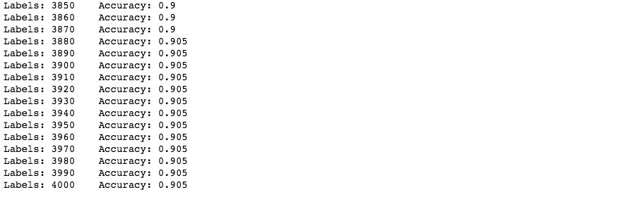
This process takes some time and gives us extra 0.8% of accuracy.

Results

Experiment Accuracy
4000 samples 92.25%
400 random samples 83.75%
400 active learned samples 89.75%
       + auto-labeling 90.50%

Conclusion

Of course, this approach has its drawbacks, like the heavy use of computation resources and the fact that a special procedure is required for data labeling mixed with early model evaluation. Also, for the testing purposes data needs to be labeled as well. However, if the cost of a label is high (especially for NLP, CV projects), this method can save a significant amount of resources and drive better project results.

This very approach has already helped us save a few thousands of dollars for one of our customers while working on the project related to Document Recognition and Classification. More details about the case can be obtained via the link.

Author:
Andy Bosyi, CEO/Lead Data Scientist MindCraft
Information Technology & Data Science

you might also like…